Bisecting Commits when Failures Are Costly October 9, 2021

This idea has been sitting in my drafts collection for several months now. About a month ago, during a 15-451 recitation, we went over a problem involving a lot of relevant ideas. I took this as a divine sign that I must finish this blog post, so here I am.

Anyway, the inspiration for this post was the git bisect command. If you’re not familiar with it, its purpose is to use binary search to determine which commit introduced a bug.¹ You tell it a known “good” commit and a known “bad” commit, and then it interactively helps you narrow down the range with a binary search until you find the first “bad” commit.

Binary search is, of course, the optimal way to search over a range, assuming your cost model is the number of queries you need to make. However, we usually aren’t actually interested in the number of queries we need to make; what interests us in the “real world” is minimizing the time taken to pick out the bad commit. In this model, is it possible to do better than binary search?

It turns out that, in theory, this is possible, although the circumstances under which such a situation would arise are not very common. The key observation is this: binary search does not distinguish between the time taken to test “good” commits and “bad” commits, minimizing only the number of commits tested. What happens if the two do not have the same cost to test? Can we contrive a scenario in which good commits cost much more to test than bad commits (or vice versa)? In such a situation, minimizing the total number of commits tested might not actually minimize the total time that the search takes!

Is such a situation possible? Well, yes, but we need to make an additional assumption: the time to test a commit is a random variable. Otherwise, say good commits cost time $t_1$ and bad commits $t_2$, where $t_1 < t_2$. We can run our test for distinguishing them, and if the time taken exceeds $t_1$, we know that the commit must be bad (and vice versa if $t_1 > t_2$). So if the testing time for each type of commit is fixed, the overall test takes only $\min\{t_1,t_2\}$ time.

On the other hand, if the times are random variables $T_1$ and $T_2$, we cannot prematurely cut off the test if we want to be sure of the outcome.² This is not so bad of an assumption: on a “real” system, the time to run some process is generally not going to be fixed, although for simple tests the randomness is probably small enough to ignore. Still, this gives us a small practical foothold, which is all I need to justify this blog post. Give a theorist an inch and he’ll take a mile.

In this setting, we can have many goals, but a reasonable one might be to minimize the expected time that the search takes. Although $T_1$ and $T_2$ are random variables, it may be the case that $E[T_1] < E[T_2]$, and so the optimal strategy is not to minimize the total number of tests made.³

In the rest of this blog post, I’ll first determine the cost of a binary search in this model. Then I’ll give another search strategy based on the classic “egg-dropping” problem, which can potentially give better results under certain assumptions on $T_1$ and $T_2$. Since I’m a computer scientist and not just a mathematician, I’ll also be writing some accompanying Haskell code to try out these different strategies. Just to get it out of the way, here are the types and primitive functions I’ll be using:

data Commit = Good | Bad deriving (Eq, Show)
data CommitSequence = Seq (Int, Int)
data Counter = Counter (Int, Int)

instance Show CommitSequence where
  show (Seq (n, k)) = show list
    where
      good = take k $ repeat Good
      bad = take (n - k) $ repeat Bad
      list = good ++ bad

instance Show Counter where
  show (Counter (good, bad)) =
    "[" ++ show good ++ " good, " ++ show bad ++ " bad queries]"

empty_counter :: Counter
empty_counter = Counter (0, 0)

-- Build a sequence of n commits where commit #k is the last "good" one.
make_commits :: Int -> Int -> CommitSequence
make_commits n k = Seq (n, k)

-- Get the number of commits in a sequence.
number_commits :: CommitSequence -> Int
number_commits (Seq (n, _)) = n

-- Query a sequence at a given index, and update a counter depending on
-- whether the commit was good or bad.
query :: CommitSequence -> Int -> Counter -> (Counter, Commit)
query (Seq (_, k)) index (Counter (good_count, bad_count)) =
  if index <= k
     then (Counter (good_count + 1, bad_count), Good)
     else (Counter (good_count, bad_count + 1), Bad)

Nothing fancy here: just a query function to make black-box queries about commits, and a Counter type to track how many good and bad commits we’ve tested so far. The code is also conveniently available in a file, so you can follow along from the comfort of your own home.

The cost of a binary search

Let’s get a little bit more formal about this. Say we have $n$ objects, some of which are of type 1 and some of which are of type 2; we know that there is a “transition point” between the type 1 and type 2 objects. If you want extra formality points⁴, define a function $f : [n] \to \{1,2\}$, where we are guaranteed that $f(1) = 1$ and $f(n) = 2$. Furthermore, we know that $f(k) = 2 \implies f(k+1) = 2$. We are allowed black-box queries to $f$, but the cost of a query is random: $$E[\text{cost to query $f(k)$}] = \begin{cases} \mu_1 & f(k) = 1 \\ \mu_2 & f(k) = 2. \end{cases}$$ We want to determine the index $k$ such that $f(k) = 1$ and $f(k+1) = 2$.

With binary search, we keep an interval $[s,t]$ where we know $f(s) = 1$ and $f(t) = 2$, and we keep on testing the midpoint of the interval. At each iteration of the algorithm, the interval halves in size, so we get a total of $\log n$ rounds.⁵

But what is the expected cost of the queries across these $\log n$ rounds? It ought to be $$\frac{\mu_1+\mu_2}{2} \log n.$$ To see this, note that if we assume that any such function $f$ is equally likely⁶, then in any given round, it is equally likely that the current query will result in $1$ or $2$. (This is because half of the possible functions $f$ that are consistent with the interval we know now will evaluate to $1$ at the midpoint, and half will evaluate to $2$.) We’re essentially taking an average over $\mu_1$ and $\mu_2$; if we truly don’t know anything about the relationship between $\mu_1$ and $\mu_2$, we can’t really do any better.

Here’s an implementation of the binary search idea, where we assume we have some black-box query function that tells us whether a commit is Good or Bad and conveniently updates a counter for us:

bisect_binary :: CommitSequence -> (Counter, Int)
bisect_binary commits =
  search empty_counter (n - 1) 0
  where
    n = number_commits commits
    search counts upper lower =
      if upper - lower <= 1
         then (counts, lower)
         else case commit of
                Good -> search counts' upper mid
                Bad  -> search counts' mid lower
      where
        mid = (upper + lower) `div` 2
        (counts', commit) = query commits mid counts

Now we can play around⁷ with this on a few different commit sequences of length, say, $n = 1000000$:

*Main> n = 1000000
*Main> bisect_binary $ make_commits n 1
([1 good, 19 bad queries],1)
*Main> bisect_binary $ make_commits n 15150
([6 good, 13 bad queries],15150)
*Main> bisect_binary $ make_commits n 789000  -- Why was 6 afraid of 7?
([11 good, 9 bad queries],789000)
*Main> bisect_binary $ make_commits n 999998
([20 good, 0 bad queries],999998)

Just to check: the index returned by bisect_binary always matches the correct answer. In each case, the exact number of good and bad commits tested differs, but they always add up to 19 (if we get really lucky) or 20. Indeed, $\log 1000000 \approx 19.932$.

Aside: a recipe for egg drop soup

We’ve seen that binary search, which does not discriminate between type 1 and type 2 objects, will make $\log n$ queries; in expectation, half of the queries will be to each type. To motivate a better strategy, let’s revisit the classic egg-dropping problem:

You are given two eggs, and you want to find the maximum floor of an $n$-story building from which you can drop an egg without breaking it. (For simplicity, assume that for any floor, either every egg dropped from that floor will break or none will.) Once you break an egg, it obviously cannot be reused, but if an egg is still intact, you can use it again. What’s your strategy for making as few guesses as possible?

This time, we cannot do a binary search over all $n$ floors. Otherwise, if we get unlucky and the first two drops break the eggs, we are out of luck. The most straightforward strategy is to just start from the first floor and work our way up until we break an egg; this takes at most $n$ guesses. But this doesn’t take advantage of the fact that we have two eggs; can we do better by allowing ourselves to break one?

If you haven’t seen this problem before, it’s a fun one, and you might want to spend a few minutes thinking about it before reading on. Below, I’ll give a solution that takes at most $2\sqrt{n}$ guesses:

1. Make evenly-spaced guesses at floors $\sqrt{n}$, $2\sqrt{n}$, $3\sqrt{n}$, and so on until you break an egg at some floor $(i+1) \sqrt{n}$.
2. Now you know that the right floor is between $i\sqrt{n}$ and $(i+1)\sqrt{n}$, so you can find the correct floor by starting from $i\sqrt{n}+1$ and working your way up every floor to $(i+1)\sqrt{n}$.

Part 1 and part 2 of this algorithm both take $\sqrt{n}$ guesses at most, so overall we will only use $2\sqrt{n}$ guesses.⁸

In fact, this same strategy gives us an algorithm using at most $kn^{1/k}$ guesses for any number $k \ge 2$ of eggs:

• If $k = 2$, just use the algorithm above.
• If $k > 2$, make $n^{1/k}$ evenly spaced guesses. Once you break an egg, repeat the algorithm with $k-1$ eggs on the interval of size $n^{(k-1)/k} = n^{\alpha}$. This takes at most $$n^{1/k} + (k-1)n^{\alpha/(k-1)} = kn^{1/k}$$ guesses, as promised.

Better than binary: bisection using egg drops

Don’t put all your eggs into one basket!

Ancient Chinese proverb⁹

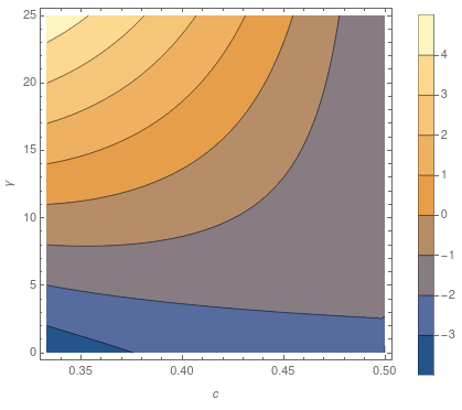
The correspondence between the egg drop problem and the commit bisection problem should be obvious. Recall that, on average, binary search used $(\log n)/2$ queries of the “slow” type. What if we use the egg-dropping strategy, allowing ourselves $k = c \log n$ slow queries, for some $c < 1/2$? We get $$k n^{1/k} = (c \log n) n^{1/(c \log n)} = (c \log n) \cdot 2^{1/c}$$ guesses in total. Concretely, suppose $\mu_1 < \mu_2$, so we allow ourselves $c \log n$ queries of type 2. (This is interchangeable with the $\mu_1 > \mu_2$ case, just by flipping the interval around.) Then this strategy gives $$\mu_2 c \log n + \mu_1 \cdot (2^{1/c} - 1)(c \log n)$$ expected cost to compute. When is this better than binary? Note that $\mu_1$ and $\mu_2$ are constant with respect to $n$; it is reasonable to suppose that the time of each query (i.e. the time to test a commit) does not depend on the length of the list (i.e. the number of commits there are). So we can define the “slowdown factor” $\gamma = \mu_2 / \mu_1 > 1$, and egg dropping will be superior, for some suitably chosen $c$, whenever $$\gamma \mu_1 c \log n + \mu_1 (2^{1/c} - 1)(c \log n) < \mu_1 \cdot \frac{1 + \gamma}{2} \log n,$$ which is the same as saying $$g(c, \gamma) = 1 + \gamma - 2c \cdot (\gamma + 2^{1/c} - 1) > 0.$$ For example, $c = 1/3$ and $\gamma = 12$ will do the trick. We can plot the areas where $g(c, \gamma) \ge 0$ using everyone’s favorite proprietary computing system, Mathematica:

f[c_, g_] := 1 + g - 2 c (g + 2^(1/c) - 1)
ContourPlot[f[c, g], {c, 1/3, 1/2}, {g, 0, 25},
  PlotLegends -> Automatic, FrameLabel -> {c, g}]

(I’ve taken the liberty of replacing “γ” with “g” above, since my code font apparently takes issue with Greek letters. I then had to rename the function from $g$ to $f$, but you get the point.) This isn’t very great, since $g(c, \gamma) > 0$ occurs only when $\gamma > 10$, or when the costly query is more than ten times the cost of the cheaper one:

This is not very likely to happen in reality, but it makes for a pretty plot. Here’s an implementation of the strategy for an arbitrary $c$:

bisect_egg :: Float -> CommitSequence -> (Counter, Int)
bisect_egg c commits =
  egg_drop empty_counter k (n - 1) 0
  where
    n = number_commits commits
    k = floor $ c * (logBase 2 $ fromIntegral n)

    -- Linear search over for first bad commit in range [lower, upper),
    -- with spacing between guesses
    search counts spacing upper lower
      | lower == upper - 1 = (counts, lower + 1)
      | lower > upper - 1 = (counts, upper)  -- Not found with this spacing
      | otherwise =
          case query commits (lower + 1) counts of
            (counts', Good) -> search counts' spacing upper $ lower + spacing
            (counts', Bad)  -> (counts', lower + 1)

    egg_drop :: Counter -> Int -> Int -> Int -> (Counter, Int)
    egg_drop counts 0 upper lower = (counts, lower)
    egg_drop counts k upper lower =
      egg_drop counts' (k - 1) upper' lower'
      where
        n' = fromIntegral $ upper - lower + 1
        spacing = floor $ n' ** (1 - (1 / fromIntegral k))
        (counts', upper') = search counts spacing upper lower
        lower' = upper' - spacing

Running them on our previous examples:

*Main> n = 1000000
*Main> c = 1/3
*Main> bisect_egg c $ make_commits n 1
([40 good, 2 bad queries],1)
*Main> bisect_egg c $ make_commits n 15150
([21 good, 6 bad queries],15150)
*Main> bisect_egg c $ make_commits n 789000
([53 good, 4 bad queries],789000)
*Main> bisect_egg c $ make_commits n 999998
([59 good, 0 bad queries],999998)

Notice that we may do many more “good” tests than binary search, but crucially, the number of “bad” tests that we run never exceeds $(\log 1000000)/3 \approx 6.644$. This tells us that, if $\gamma$ is high enough, we should be beating binary search on average.

Corrigendum: an earlier version of this post had an incorrect implementation of the egg dropping routine; I forgot to update the length of the interval, which led to many more iterations than needed. I’m still not 100% sure that the indexing is correct, but it is much better now.